Quantum readiness: Lattice-based PQC

Lattices are mathematical constructions playing a significant role in cryptography. They are used for constructing various cryptographic tools such as asymmetric encryption schemes, hash functions, key exchanges, signatures, and homomorphic encryption. They are also great tools for analyzing existing cryptosystems that are not necessarily originally constructed on hard lattice problems.

Introduction to Lattices

What's a lattice ?

"A set of regularly spaced points." This very broad (and informal) definition of a lattice captures the image of what we call a lattice; it can be a simple grid of squares; it can be the atomic structure of crystals; it can even appear on the top of pies!

One of the simplest lattice you can think of is the square lattice:

Actually there's an even simpler lattice you can make: integers on the number line !

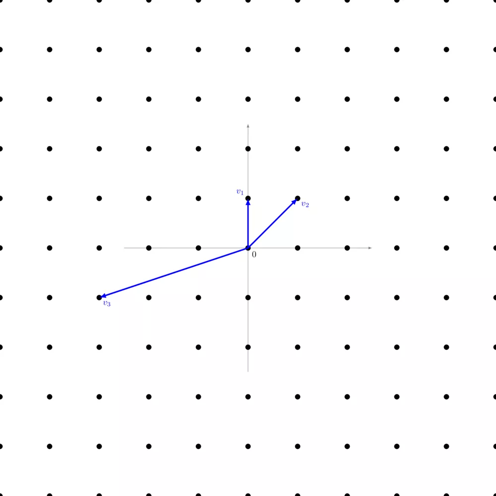
More formally, a lattice $\Lambda$ is the set of linear combinations with integer coefficients of a family of linearly independent vectors. Let $( b_1,…,b_n )$ be a family of linearly independent vectors of $\mathbb{R}^n$, then we can form a lattice: \begin{align} \Lambda = \left\{ \sum^n_{i=1} a_i b_i | a_i \in \mathbb{Z} \right\} \end{align}

On the picture right above, we have $v_1 = \left( \begin{smallmatrix} 1 & 0 \end{smallmatrix} \right)$, $v_2 = \left( \begin{smallmatrix} 1 & 1 \end{smallmatrix} \right)$, and $v_3 = \left( \begin{smallmatrix} -3 & -1 \end{smallmatrix} \right)$. Just like in a vector space, you can add two vectors, calculate their opposite, multiply them by a scalar, and there's a zero vector at the origin. The only constraint is that scalars must be in integers.

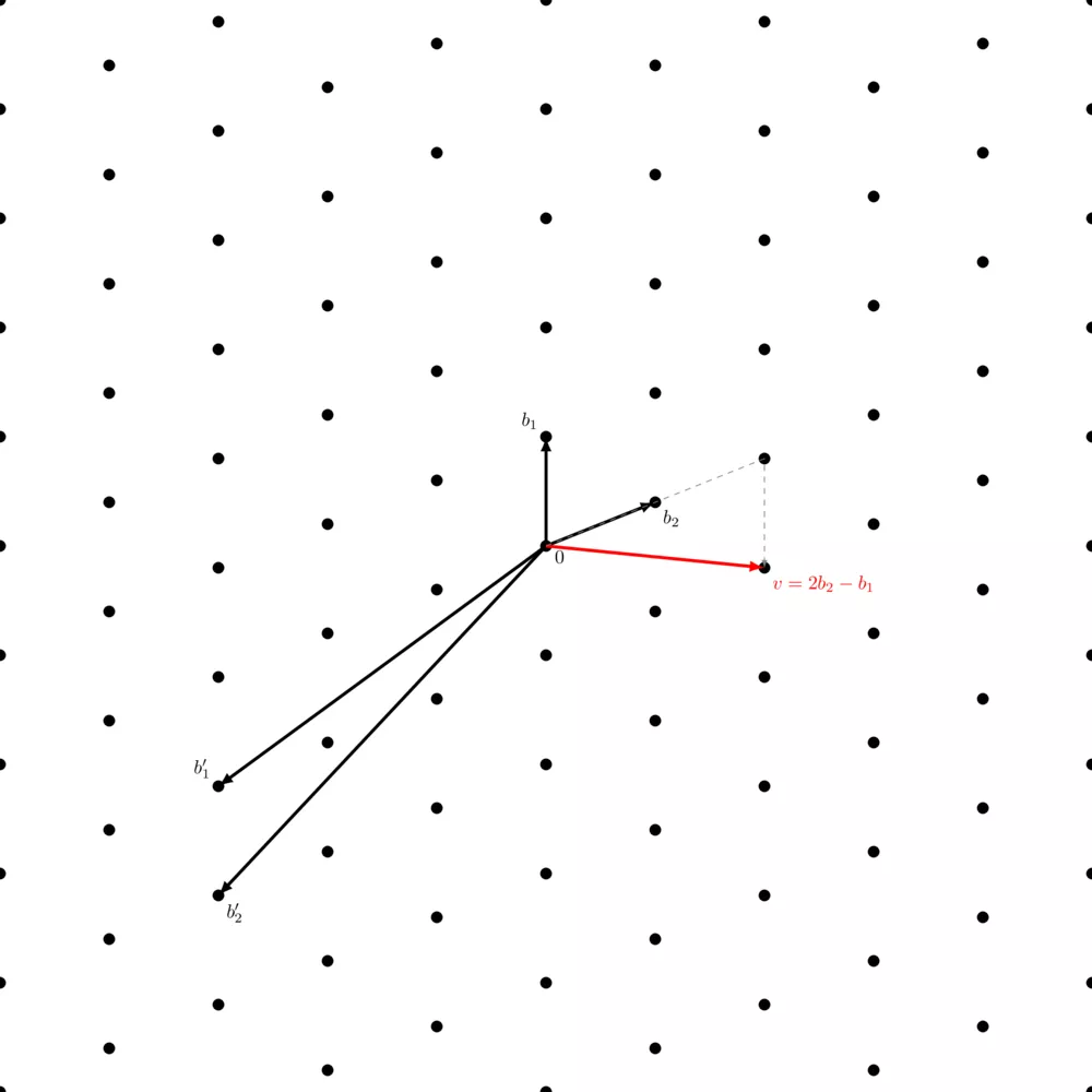
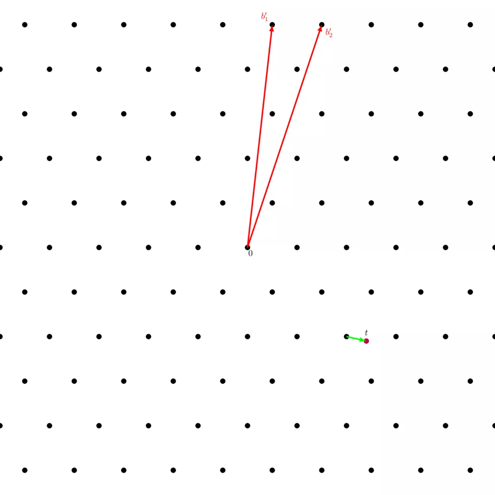
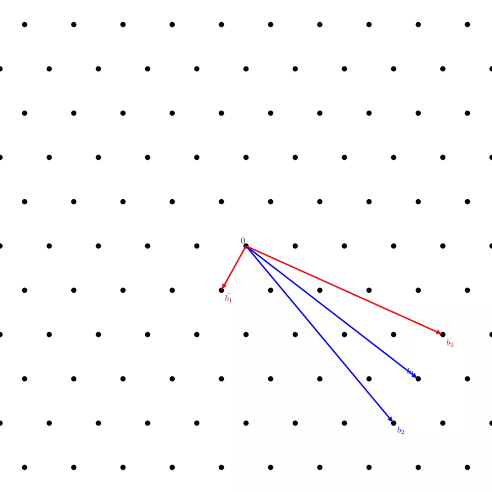
You can notice that in the above picture, the lattice generated by $( b_1, b_2 )$ and the one generated by $( b'_1, b'_2 )$ is the same. It's simply somewhat harder to visualize how the set of integer linear combinations of $( b'_1, b'_2 )$ generates all these points.

However, not any two linear independent vectors of this lattice generate the same lattice:

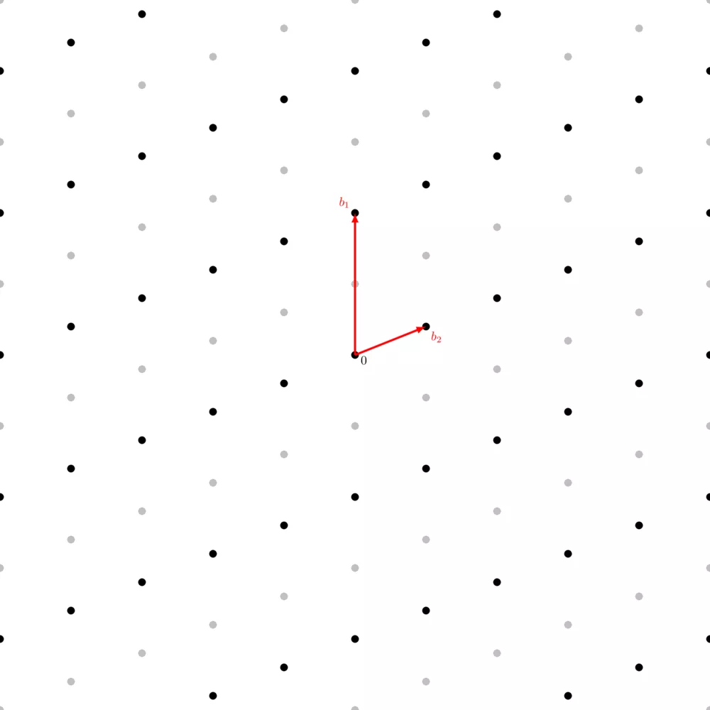
It looks like it's the same lattice, just because the points of the previous lattice are left out, but it's not the same. The point halfway through $b_1$ which was reachable in the previous lattice, is now unreachable by a linear combination of these vectors (remember, scalars are only integers, so no multiplying this new $b_1$ with $0.5$).

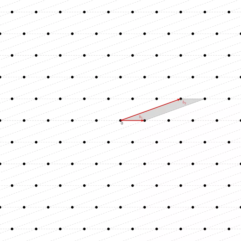
The Fundamental Parallelepiped

The fundamental parallelepiped or fundamental domain of a lattice $\Lambda$ with basis $B = ( b_0, ..., b_n )$ is defined as

\begin{align} \mathcal{F}(B) = \left\{ \sum a_i b_i \mid 0 \leq a_i < 1 \right\} \end{align}

Intuitively, you can picture it as the set of points that are reachable via a linear combination of the basis vectors but without extending them, only shrinking them ($a_i < 1$). This means that the origin is the only point contained in the fundamental parallelepiped. Here's how it looks like:

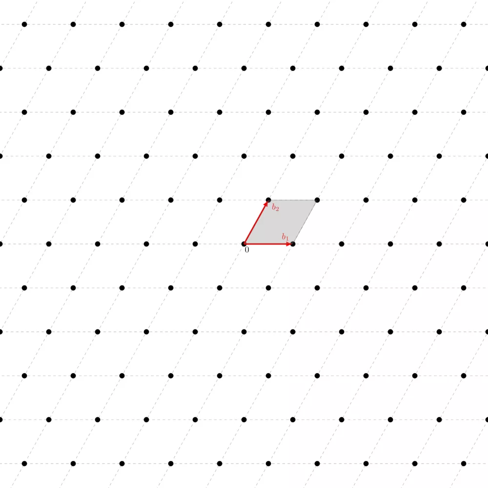
You can see how you can tile the whole plane using this same parallelepiped. The area of the fundamental parallelepiped is what we call the volume of the lattice $\text{vol}(\Lambda) = \text{vol}(\mathbb{R} / \Lambda) = |\text{det}(\Lambda)|$. We call this measure the volume of the lattice, or its co-volume, or its determinant. The nice thing with this is that whatever the basis of the same lattice you have, the volume of its fundamental parallelepiped is always the same.

This property is very important, for many reasons, one of them being that we have this powerful theorem called Minkowski's theorem which sets an upper bound on what we call the "first minimum" of the lattice, $\lambda_1(\Lambda)$, which corresponds to the length of the shortest vector of the lattice. Minkowski's theorem basically says that every convex shape $S$ (convex just means that for any two points you take on $S$, the segment that links them only goes through $S$, it doesn't pass outside the shape) which is symmetric (for any point on $S$, its opposite is also on $S$), if $\text{vol}(S) > 2^n \text{vol}(\Lambda)$, then $S$ necessarily contains at least one nonzero point. One corollary, which is of particular interest in lattice-based cryptography, is that $\lambda_1(\Lambda) \leq \sqrt{n} |\text{vol}(\Lambda)|^{\frac{1}{n}}$ where $n$ is the lattice's dimension.

This fact can be very useful both for analyzing lattice-based cryptosystems, but also when trying to map an existing problem to the problem of finding a vector with length $\lambda_1(\Lambda)$ given a basis with very long vectors. Speaking of which, let's introduce what is probably the most famous lattice problem widely used in cryptography.

Shortest Vector Problem

One of the most important hard lattice problems is called the "shortest vector problem" ($\mathsf{SVP}$). It consists of being given a basis of the lattice and finding a nonzero shortest vector, a vector of length $\lambda_1(\Lambda)$. We note "a nonzero shortest vector" because there are at least two vectors of length $\lambda_1(\Lambda)$, one and its opposite.

This problem is conjectured to be NP-hard. Keep in mind that all lattices shown here are 2-dimensional lattices simply because they're easier to understand, but lattices used in lattice-based cryptographic schemes typically have between 400 to 1000 dimensions.

The issue with using $\mathsf{SVP}$ is that it is a hard problem in the worst case. We need problems that are hard on average, i.e., by sampling a random instance of the problem, this instance is hard with a very high probability.

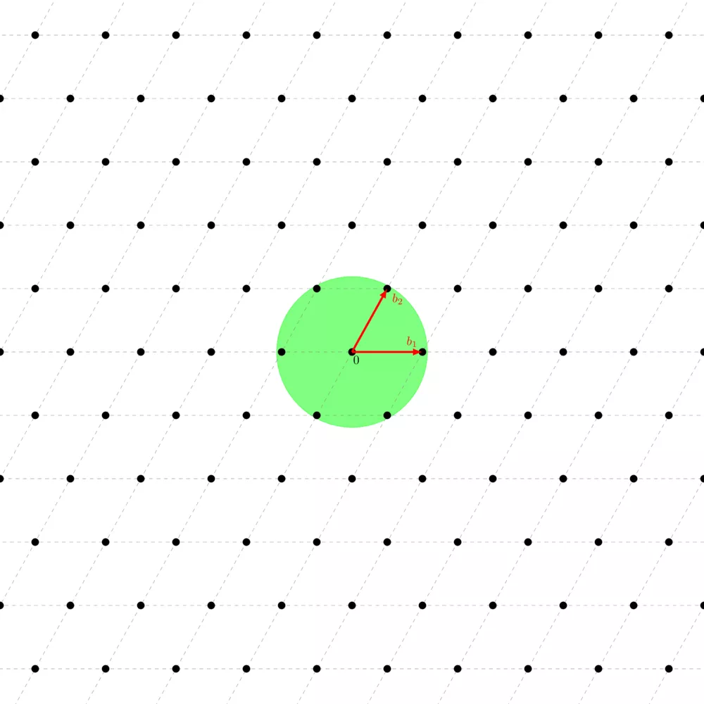
Approx-SVP

$\alpha-\mathsf{approx-SVP}$ is basically the same but easier. We define a factor $\alpha$, from which we define a circle at the origin of radius $\alpha \cdot \lambda_1(\Lambda)$. Each lattice point within the circle counts as a solution to the $\alpha-\mathsf{approx-SVP}$, even if it's not a valid solution to the shortest vector probleù.

Unique-SVP

The $\delta-\mathsf{uSVP}$ is closely related to $\mathsf{SVP}$, but with the additional constraint that the shortest non-zero vector is unique (or nearly unique) compared to all other lattice vectors by a factor of at least $\delta$. This problem, like $\mathsf{SVP}$, is conjectured to be hard as the dimension $n$ grows.

Shortest Independent Vectors Problems

The Shortest Independent Vectors Problems ($\mathsf{SIVP}$) is just like the $\mathsf{SVP}$, but the problem now consists of finding $n$ short, linearly independent vectors in the lattice. Much like the $\mathsf{SVP}$, the $\mathsf{SIVP}$ also has an approximate version, called the $\gamma-\mathsf{SIVP}$.

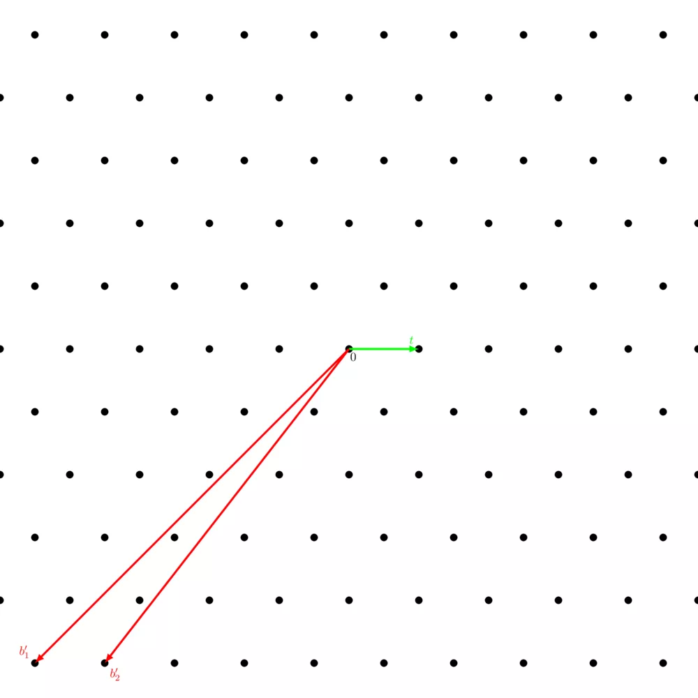
Closest Vector Problem

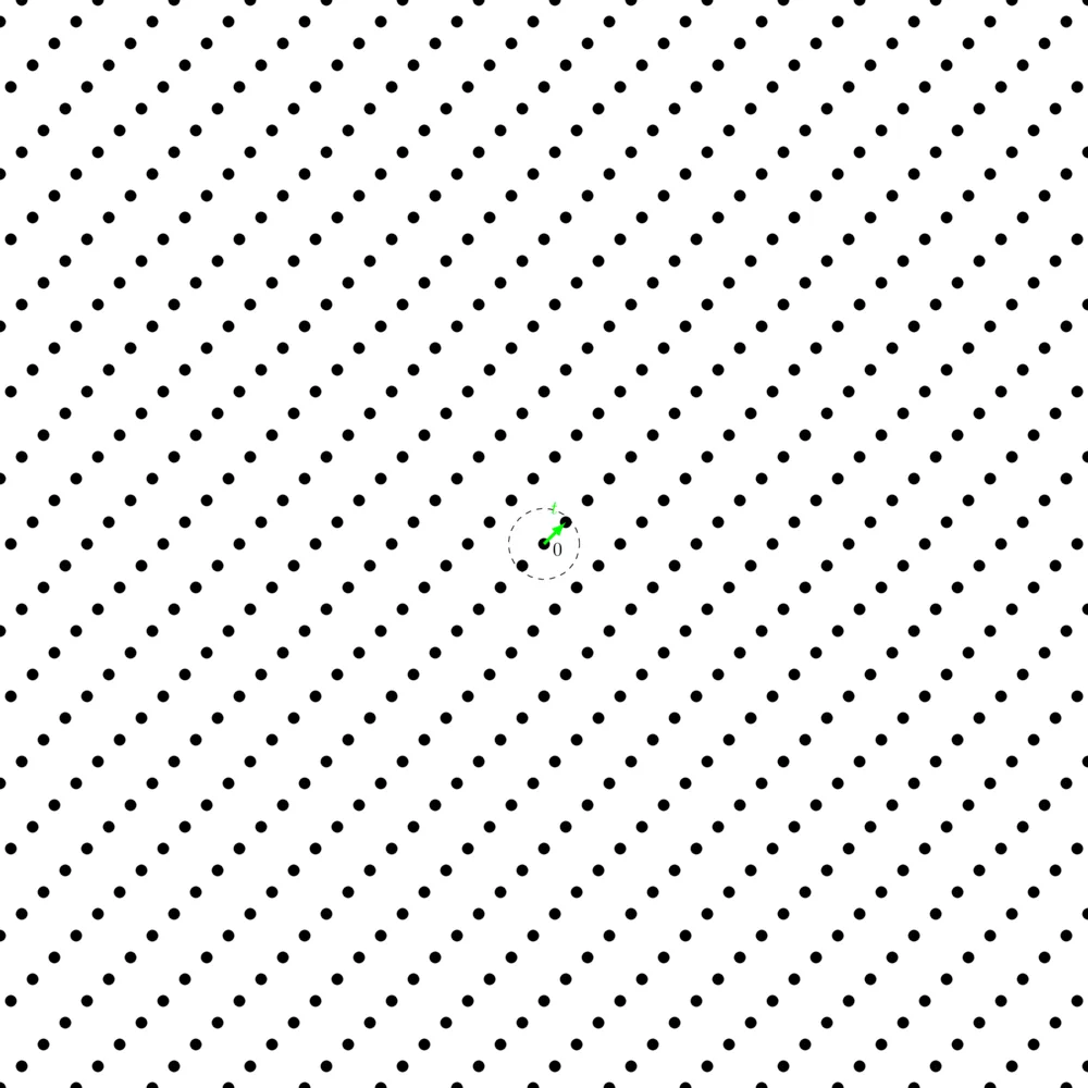
The closest vector problem ($\mathsf{CVP}$) is also one of the two main hard lattices problems. It consists of being given a basis and a point on the real space (which isn't on the lattice), and finding its closest point on the lattice.

Just like the $\mathsf{SVP}$, the $\mathsf{CVP}$ is only hard in the worst case.

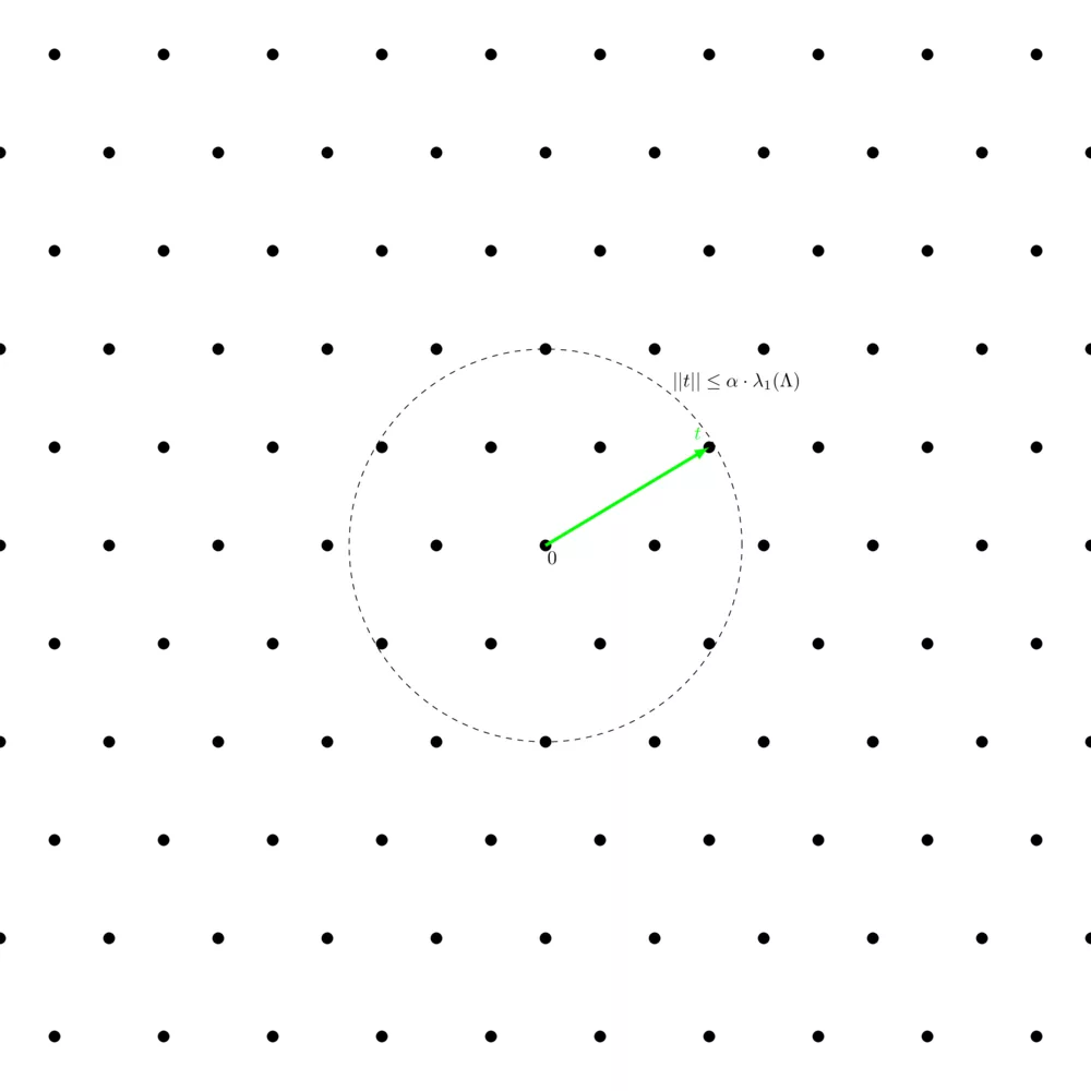
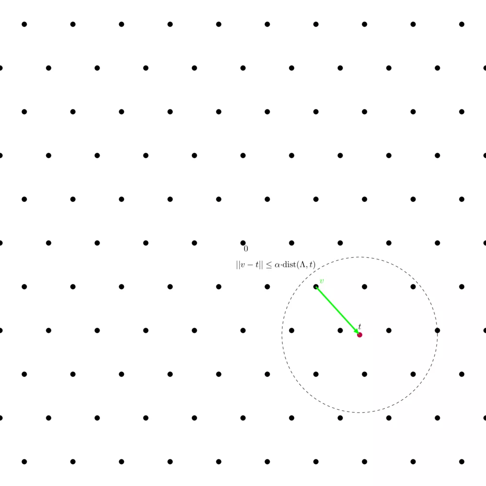
Approx-CVP

$\alpha-\mathsf{approx-CVP}$ is basically the same but easier - again. We define a factor $\alpha$ from which we define a circle at $t$ of radius $\alpha \cdot \text{dist}(\Lambda, t)$, where $\text{dist}(\Lambda, t)$ denotes the distance of $t$ to the closest lattice point. Each lattice point within the circle counts as a solution to the $\alpha-\mathsf{approx-CVP}$.

Bounded Distance Decoding

$\delta-\mathsf{BDD}$ is closely related to $\mathsf{CVP}$, but the key difference is that, in $\mathsf{BDD}$, the target point is guaranteed to be within a certain bounded distance (defined by $\delta$) from the lattice. This guarantee is what makes the problem distinct from $\mathsf{CVP}$. Much like $\delta-\mathsf{uSVP}$, $\delta-\mathsf{BDD}$ is conjectured to be hard as the dimension $n$ grows.

Quantum Resilience

As it turns out many of these lattice-based problems, including the Shortest Vector Problem ($\mathsf{SVP}$), $\mathsf{approx-SVP}$, $\mathsf{unique-SVP}$, Shortest Independent Vectors Problem ($\mathsf{SIVP}$), Closest Vector Problem ($\mathsf{CVP}$), and Bounded Distance Decoding, are considered quantum resilient. This means they are believed to maintain their computational hardness even against attacks using quantum computers, making them particularly valuable for post-quantum cryptographic systems.

$q$-ary lattices

A $q$-ary lattice is a type of lattice that is particularly important in the field of lattice-based cryptography. It's defined over a finite field with $q$ elements, typically a prime number or a power of a prime. $q$-ary lattices behave exactly like the infinite lattices we've seen so far, except that the component of every vector is taken modulo $q$. More formally, a $q$-ary lattice is a lattice that can be constructed by taking all integer linear combinations of the rows of a matrix $A$ over $\mathbb{Z}$, where the rows of $A$ belong to $\mathbb{Z}^n_q$ (the set of $n$-dimensional vectors over the finite field with $q$ elements). We denote such a lattice by $\Lambda_q(A)$.

$q$-ary lattices are crucial in constructing problems that are hard on average. Two widely used of these problems are the Short Integer Solution ($\mathsf{SIS}$) problem along with the Learning With Errors ($\mathsf{LWE}$) problem that we'll see later on.

Lattice Reductions

This section builds its way to what's probably the most famous algorithm in lattice studies, the LLL algorithm. First we'll need to introduce the Gram-Schmidt algorithm for creating orthogonal bases, then we'll introduce the concept of weakly reduced bases and of reduced bases, and then we'll see what the LLL algorithm is all about.

Gram-Schmidt Orthogonalization

Given a basis $B = ( b_1, \dots, b_m )$ of the lattice $\Lambda$ of dimension $n$, where $1 \leq m \leq n$, we say that the basis $B$ is orthogonal if for all $1 \leq i \leq j \leq m$, $\langle b_i, b_j \rangle = 0$, where $\langle \cdot, \cdot \rangle$ denotes the dot product. The Gram-Schmidt Orthogonalization procedure produces an orthogonal basis $B^*$ of the same lattice $\Lambda$ given $B$:

1. $b^*_1 \leftarrow b_1$
2. $\texttt{for } i = 2, \dots, m \texttt{ do}$

\begin{align} & \mu_{ij} \leftarrow \frac{\langle b_i, b^*_j \rangle}{\langle b^*_j, b^*_j \rangle}, \hspace{20px} 1 \leq j \leq i-1 \\ & b^*_i \leftarrow b_i - \sum^{i-1}_{j=1}\mu_{ij} \cdot b^*_j \end{align}

In typical linear algebra courses, when teaching students about the Gram-Schmidt algorithm, each $b^*_i$ is divided by its norm in order for the algorithm to produce an orthonormal basis. We don't do that that here as it will have a counter productive effect on lattice basis reduction for reasons that will become obvious in the next few sections of this chapter.

For example, running Gram-Schmidt on $B = \begin{pmatrix} 4 & -2 \\ \frac{19}{5} & -1 \end{pmatrix}$ yields $B^* = \begin{pmatrix} 4 & -2 \\ \frac{9}{25} & \frac{18}{25} \end{pmatrix}$:

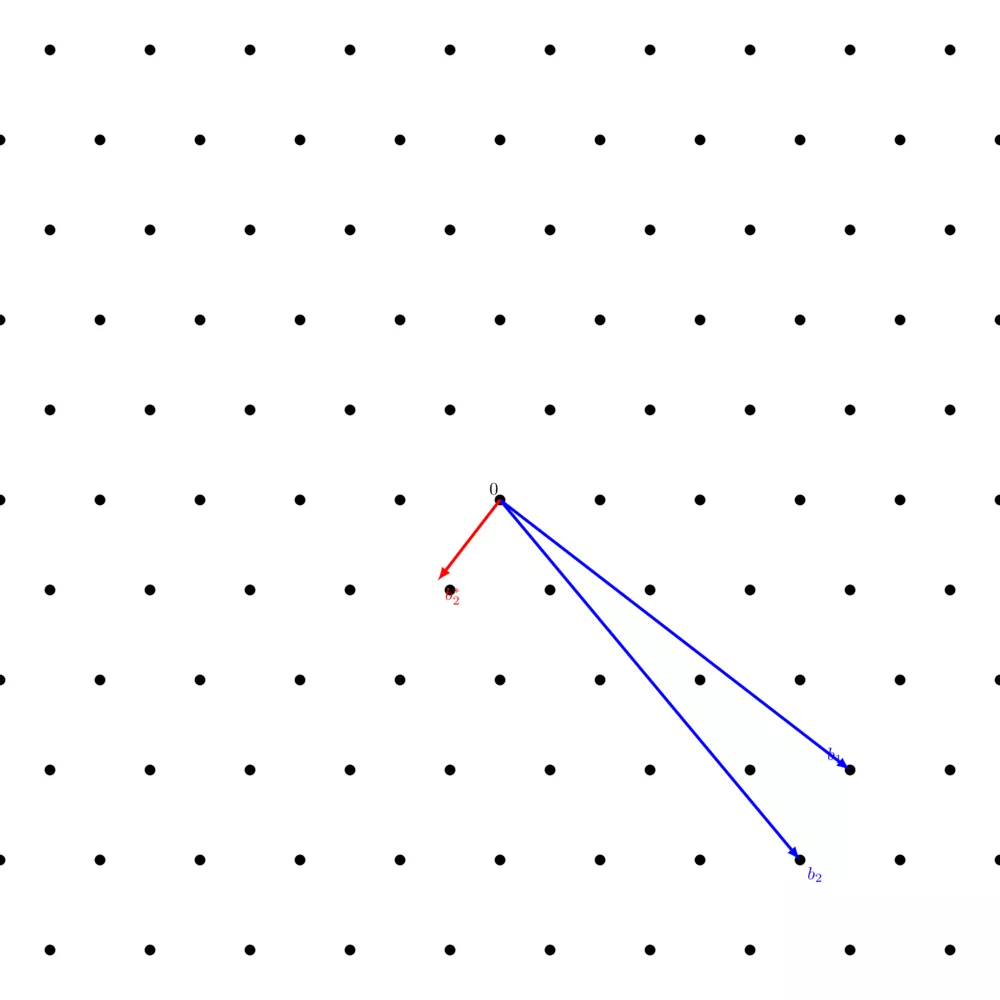
$b_1$ is left unchanged and $b_2$ yielded $b^*_2$ which is orthogonal to $b_1$, but you'll notice that $b^*_2$ is not on the lattice. That's because, in the general case, $\Lambda(b_1, \dots, b_n) \neq \Lambda(b^*_1, \dots, b^*_n)$ because most lattices do not have any orthogonal basis.

The reader is highly encouraged to visualize the Gram-Schmidt process for $n = m = 2$ and $3$, there a nice animation of it on the Wikipedia page.

Weak Reduction

We say that a basis is weakly reduced iff: if we were to orthogonalize it with the Gram-Schmidt procedure, we'd have $|\mu_{ij}| \leq \frac{1}{2}$ for all $i, j$. Notice that if the input basis of the Gram-Schmidt procedure has vectors that are orthogonal two-by-two, we'd have $|\mu_{ij}| = 0$ for all $i, j$, intuitively meaning that a weakly reduced basis is a basis that is almost orthogonal i.e. that is orthogonal with a precision of $\frac{1}{2}$. We now define the algorithm $\texttt{WeakReductionStep}$ which takes in a basis $B = (b_1, \dots, b_n)$ and outputs a basis $\bar{B} = (\bar{b_1}, \dots, \bar{b_n})$ of the same lattice:

1. $\texttt{Initialize } \bar{B} \leftarrow B \texttt{.}$
2. $B^* \leftarrow GramSchmidt(B)$. $\texttt{Let } \mu_{ij} \texttt{ be the coefficients used in the Gram-Schmidt procedure.}$
3. $\texttt{If for all } (i,j), |\mu_{ij}| \leq \frac{1}{2} \texttt{, return B.}$
4. $\texttt{Let } (i_0,j_0) \texttt{ be the largest pair in lexicographical order s.t. } |\mu_{i_0 j_0}| > \frac{1}{2} \texttt{.}$
5. $\texttt{Let } c_0 = \lfloor \mu_{i_0 j_0} \rceil \texttt{ the closest integer to } \mu_{i_0 j_0} \texttt{.}$
6. $\bar{b_{i_0}} \leftarrow b_{i_0} - c_0 b_{j_0}$
7. $\texttt{Return } \bar{B} \texttt{.}$

Using the $\texttt{WeakReductionStep}$, given a basis $B = (b_1, \dots, b_n)$, we can obtain a weakly reduced basis $\bar{B} = (\bar{b_1}, \dots, \bar{b_n})$ of the same lattice by constructing the following algorithm $\texttt{WeakReduction}$:

1. $\texttt{Initialize } \bar{B} \leftarrow B \texttt{.}$
2. $\texttt{While } \bar{B} \texttt{ is not weakly reduced, } \bar{B} \leftarrow \texttt{WeakReductionStep}(\bar{B}) \texttt{.}$
3. $\texttt{Return } \bar{B} \texttt{.}$

    

You can visualize the process of $\texttt{WeakReduction}$ just like you visualized the Gram-Schmidt process, except that instead of scaling $b^*_j$ by $\mu_{ij}$, you scale it by the integer that is the closest to $\mu_{ij}$.

LLL Algorithm

The LLL algorithm is a lattice reduction algorithm that runs in polynomial time. It gets its name from the three mathematicians who came up with it, Arjen Lenstra, Hendrik Lenstra, and László Lovász. But before defining it, we first need to talk about reduced bases. We say that a basis is reduced iff it is weakly reduced, and if it satisfies:

\begin{align} || b^*_i ||^2 \leq 2|| b^*_{i+1} ||^2 \end{align}

Where $B^* = (b^*_1, \dots, b^*_n)$ is its Gram-Schmidt version. This inequality is a simplified form of what we call the Lovász condition. From this link, we read

It seems that Lenstra, Lenstra, and Lovász have noticed that a situation in which length reduction alone is stuck with a very bad basis — as depicted in the first image — always has vectors which are in the "wrong" order comparing their lengths and which are far from being orthogonal, and that it helps in this case to exchange them and continue length-reducing. That is really the core idea of the LLL algorithm.

Even though the image from the above link isn't displayed here, you can arrive at the same conclusion using the previous image of this article. $b_2$ is reduced by comparing with $b_1$, but what about reducing $b_1$ ? The "stuck with a very bad basis" occurs here only once since we're in 2 dimensions, but it can occurs many times in higher dimensions. We thus add the $\texttt{ReductionStep}$ procedure that simply exchanges/swaps two columns $i$ and $i+1$ that doesn't match the Lovász condition. The choice of $i$ is not unique.

Here's the LLL algorithm:

1. $\texttt{Initialize } \bar{B} \leftarrow \texttt{WeakReduction}(B) \texttt{.}$
2. $\texttt{While } \bar{B} \texttt{ is not reduced, do }$

   \begin{align} & \bar{B} \leftarrow \texttt{ReductionStep}(\bar{B}) \\ & \bar{B} \leftarrow \texttt{WeakReduction}(\bar{B}) \texttt{.} \end{align}

Applying the LLL algorithm on the same basis as in the above picture, we get:

You can notice how, in comparison with the $\texttt{WeakReduction}$ algorithm, $\bar{b_1}$ and $\bar{b_2}$ were swapped which allowed to also reduce the very long vector ($\bar{b_1}$ in the previous picture, $\bar{b_2}$ in this one) and make it more orthogonal to the newly found short vector ($\bar{b_1}$ in the previous picture, $\bar{b_2}$ in this one).

It's important to note that the LLL presented here is only in it's most basic form in order for the reader to better grasp the intuition of the algorithm. The "simple Lovász condition" can be improved by the "real Lovász condition": \begin{align} \delta || b^*_{i-1} ||^2 \leq || b^*_{i-1} + \mu_{i,i-1} b^*_{i-1} || \end{align}

where the parameter $\delta$ must satisfy $0.25 \leq \delta \leq 1$ is order to guarantee polynomial-time execution of the algorithm. Make $\delta$ less than $1/4$ and the algorithm might enter a loop where it continuously swaps and adjusts vectors without ever arriving at a "reduced" basis according to the algorithm's criteria. Make $\delta > 1$ and the algorithm might stall or fail to find a basis that satisfies this condition. In SageMath $\delta$ is set to $0.99$ by default and Magma's default is $\delta = 3/4$. There are several other modifications to make to our LLL algorithm in order for it to be complete but this is beyond the scope of the article. You can see the original LLL algorithm in the original paper 1.

Learning With Errors

Imagine that you're given a system of linear equation to solve over the integers but each line has a little constant, a little noise/error, added to it that you don't know (you just know it's there). You're tasked to give the solution to the system. That's what $\mathsf{LWE}$ basically is.

$\mathsf{LWE}$ is a foundational problem in lattice-based cryptography, introduced by Oded Regev in 2005 2. It underpins the security of various cryptographic protocols by leveraging the hardness of solving certain lattice problems in the presence of noise. Regev's formulation has been pivotal in advancing the development of quantum-resistant cryptographic systems.

More formally, let

\begin{align} & q \text{ a prime.} \\ & \chi \text{ a probability distribution on } \mathbb{Z}_q. \\ & \mathbf{A}_{s,\chi} \text{ the probability distribution obtained by choosing a vector } \mathbf{a} \in \mathbb{Z}^n_q \text{ uniformly at random,} \\ & \hspace{25px} \text{choosing } \mathbf{e} \in \mathbb{Z}_q \text{ according to } \chi \text{, and outputting } (\mathbf{a}, \langle \mathbf{a}, \mathbf{s} \rangle + \mathbf{e}). \end{align}

Given an arbitrary number of samples from the probability distribution $\mathbf{A}_{s,\chi}$, the goal is to recover the secret $\mathbf{s}$. The choice of the parameters $q$, $n$, and the distribution $\chi$ affects both the security and efficiency of the $\mathsf{LWE}$ problem. Typically, $\chi$ is chosen to be a Gaussian distribution.

Recovering $\mathbf{s}$ from $\mathbf{A}_{s,\chi}$ is the search variant of the problem which you can reduce to the decision variant for evaluating cryptosystems based on $\mathsf{LWE}$. The decision variant consists of trying to distinguish samples from $\mathbf{A}_{s,\chi}$ from uniformly chosen samples, much like distinguishability games we saw in the first article.

As said above, $\mathsf{LWE}$ relies on systems of linear equations over the integers. We can reformulate the problem to make the connection to $q$-ary lattices obvious, by being given

\begin{align} \left( A, b = A \cdot s + e \mod q \right) \ \end{align}

and solving

\begin{align} A \cdot s \thickapprox b \mod q \end{align}

Where $A$ is the matrix containing the $\mathbf{a}$ vector of each sample from $\mathbf{A}_{s,\chi}$. It is also easy to see that $b$ is a vector containing the second element of each samples from $\mathbf{A}_{s,\chi}$ as its coefficients.

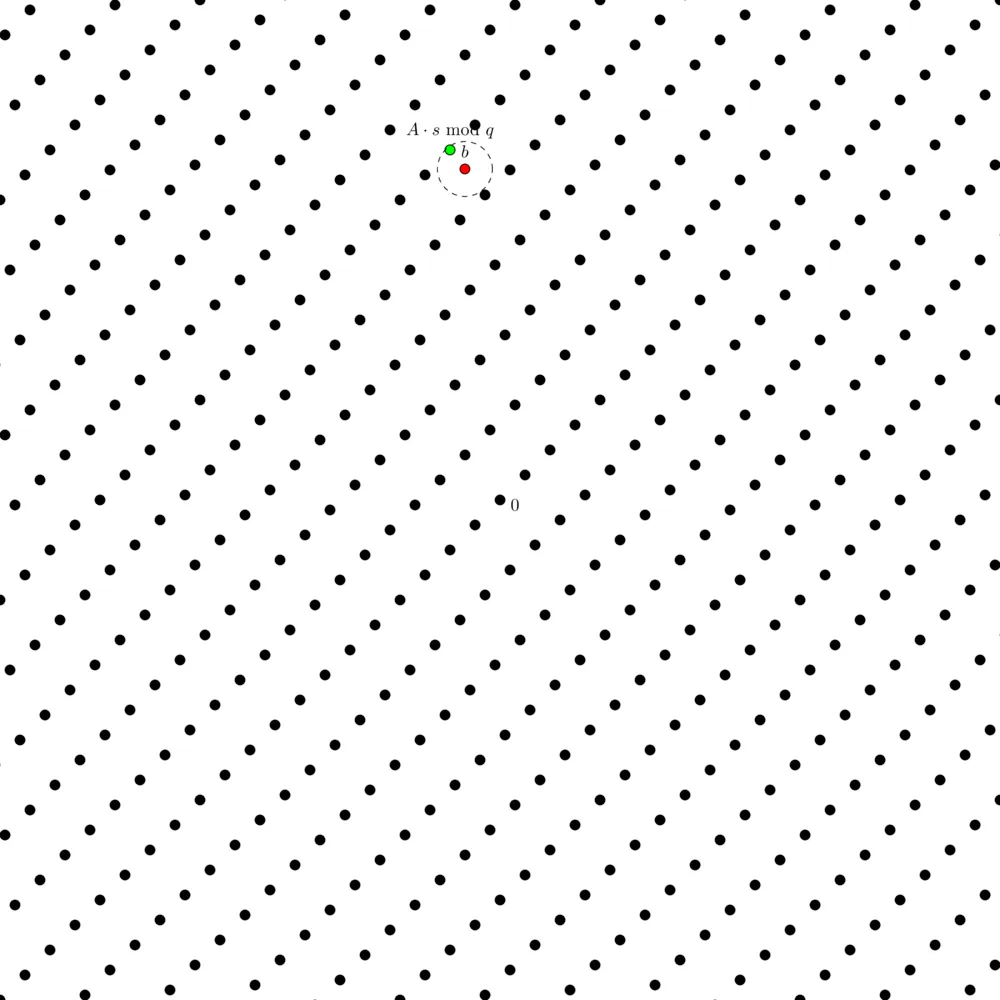
From an $\mathsf{LWE}$ instance with a small error $e$, we can form a $\mathsf{BDD}$ instance in the lattice $\Lambda_q(A)$ and try to find a lattice point $v = A \cdot s \mod q$ from a non-lattice point $b = v + e$.

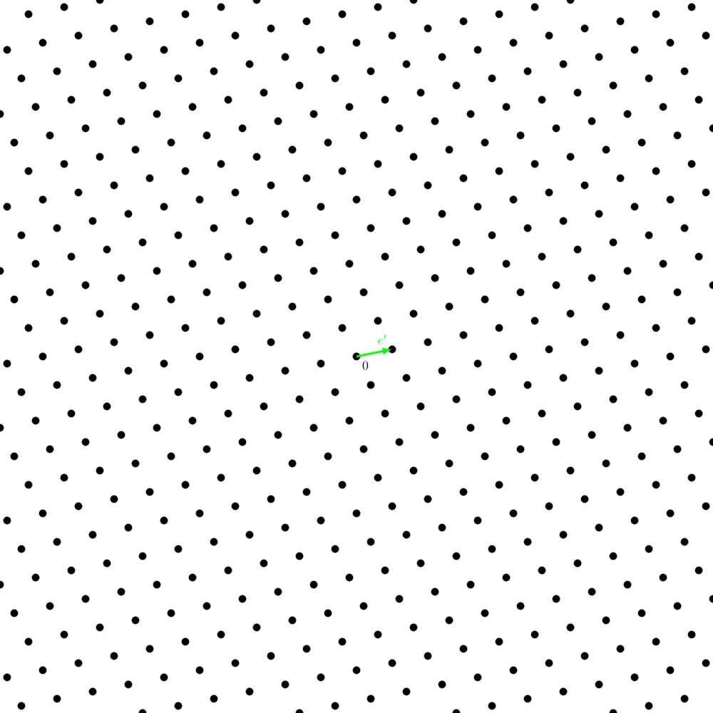
We can also get an $\mathsf{uSVP}$ instance from an $\mathsf{LWE}$ instance by building a lattice $\Lambda_q \left(\begin{pmatrix} A & b \\ 0_n & 1 \end{pmatrix} \right)$ where the shortest vector is $e' = (e, 1)$.

Solving the $\mathsf{BDD}$ problem for any lattice is at least as hard as solving $\mathsf{LWE}$ with non-negligible probability, which is itself at least as hard as solving the $\mathsf{approx-SVP}$ in any lattice.

Oded Regev has put forward an asymmetric encryption scheme based on the $\mathsf{LWE}$ assumption (the assumption that solving the $\mathsf{LWE}$ problem is hard), which he himself declared to be inefficient and without any real-world use3. It is only a proof of concept.

The cryptosystem is parameterized by several integers:

• $n$: the security parameter,
• $m$: the number of equations (specifically $m = 1.1 \cdot n \cdot \log q)$,
• $q$: the modulus, chosen to be a prime between $n^2$ and $2n^2$,
• $\alpha$: the noise parameter, set as $\alpha = 1 / \left( \sqrt{n \cdot \log^2 n} \right)$.

The system involves typical key generation, encryption, and decryption processes:

• Key Generation ($Gen$): the key generation algorithm which outputs a private key $s$ and a public key $(a_i, b_i)^m_{i=1}$. $s$ is a vector chosen uniformly from $\mathbb{Z}^n_q$, the $n$-dimension space of integers modulo $q$, and $(a_i, b_i)^m_{i=1}$ consists of $m$ samples from $\mathbf{A}_{s,\chi}$ additionally parameterized by the modulus $q$ and the error parameter $\Delta$. $m$ represents here the number of equations.
• Encryption ($Enc$): takes in a message $m$ and outputs a tuple $c$. For each bit $m_i$ of $m$, a random set $S$ is chosen uniformly among all $2^m$ subsets of $\left\{ 1, 2, \dots, m \right\}$, and \begin{align} c_i = \begin{cases} \left( \sum_{i \in S} a_i, \sum_{i \in S} b_i \right), && \text{if } m_i = 0 \\ \left( \sum_{i \in S} a_i, \lfloor \frac{q}{2} \rfloor + \sum_{i \in S} b_i \right), && \text{if } m_i = 1 \end{cases} \end{align}
• Decryption ($Dec$): takes in a ciphertext $c$ consisting of tuples of the form $(a, b)$ and outputs the concatenation of the bits $m_i$ defined by: \begin{align} m_i = \begin{cases} 0, && \text{if } (b - \langle a, s \rangle) \text{ modulo } q \text{ is closer to } 0 \text{ than it is to } \lfloor \frac{q}{2} \rfloor \\ 1, && \text{otherwise} \end{cases} \end{align}

The public key size and the message size during encryption scale as $O(n \log q)$, leading to significant storage and computational overhead, particularly because $m = 1.1 \cdot n \log q$. Decryption correctness relies on the error component being manageable, i.e., the accumulated error in $\mathsf{LWE}$ samples does not exceed $q/4$, which is typically negligible under standard parameters.

The security proof is based on the LWE assumption, defending against chosen plaintext attacks. It asserts that distinguishing between $\mathsf{LWE}$ samples and uniform samples implies solving the $\mathsf{LWE}$ problem, therefore using the problem's hardness to secure the cryptosystem. A formal security proof involves showing that the distribution of encrypted messages cannot be efficiently distinguished from a uniform distribution unless the underlying $\mathsf{LWE}$ problem can be solved, leveraging $\mathsf{LWE}$ hardness.

Short Integer Solution problem

The Short Integer Solution ($\mathsf{SIS}$) problem is a fundamental challenge in lattice-based cryptography and was introduced by Miklós Ajtai in a seminal paper which also established the average-case hardness of certain lattice problems based on the worst-case hardness of others 4. The formal definition of the $\mathsf{SIS}$ problem can be presented as follows:

Let $n$, $m$, $q$ be positive integers and $\beta$ a positive real number. Consider a uniformly random matrix $A \in \mathbb{Z}_q^{n \times m}$. The SIS problem is defined as finding a non-trivial vector $x \in \mathbb{Z}^m$ such that:

1. $Ax = 0 \mod  q$
2. $||x|| \leq \beta$

where $||x||$ denotes some norm of $x$, typically the Euclidean norm.

The complexity of the $\mathsf{SIS}$ problem depends on the choice of parameters. It is widely believed to be hard when $q$ is polynomial in $n$ and $\beta$ is set in such a way that the solution is non-trivial and difficult to find. The problem's hardness is conjectured based on the worst-case hardness of finding short vectors in random lattices, specifically relating to the $\mathsf{SVP}$.

Ajtai's Hash Functions

Building on the foundation of the SIS problem, Miklós Ajtai introduced a hash function that is provably collision-resistant based on the hardness of the $\mathsf{SIS}$ problem. The hash function is constructed as follows:

1. Setup: Select a random matrix $A$ from $\mathbb{Z}_q^{n \times m}$ as described above.
2. Hash Function: The hash of a message $\mathbf{m} \in \{0,1\}^m$, represented as a binary vector of length $m$, is computed by $H(\mathbf{m}) = A \mathbf{m} \mod  q$.

A collision in this hash function occurs when two distinct messages $\mathbf{m}$ and $\mathbf{m'}$ satisfy $H(\mathbf{m})=H(\mathbf{m'})$. This implies that $A(\mathbf{m}−\mathbf{m'})=0 \mod  q$, and $\mathbf{m}−\mathbf{m'}$ is a non-zero solution to the SIS problem with $\beta = \sqrt{\frac{m}{2}}$ in the average case, given by a counting argument on the number of non-zero entries in $\mathbf{m}−\mathbf{m'}$:

• Each message $\mathbf{m}$ and $\mathbf{m'}$ is represented as a binary vector of length $m$. The vector resulting in their difference, $\mathbf{d} = \mathbf{m} - \mathbf{m'}$, has as components either $0$ if $m_i = m'_i$, $1$ if $m_i = 1$ and $m'_i = 0$, and $-1$ if $m_i = 0$ and $m'_i = 1$.
• Assuming $\mathbf{m}$ and $\mathbf{m'}$ are independent and randomly chosen, the probability of a specific entry $d_i$ being nonzero ($1$ or $-1$) occurs with a probability of $1/2$.
• Since the norm $||\mathbf{d}||$ is the sum of the square of the non-zero entries, each nonzero entry contributes to $1$ to the norm, thus $||\mathbf{d}||$ is approximately $\sqrt{\frac{m}{2}}$.

The collision-resistance of Ajtai's hash function directly relates to the difficulty of solving the $\mathsf{SIS}$ problem. If the $\mathsf{SIS}$ problem is hard for the given parameters, then finding a collision in the hash function is also hard, thus ensuring its security.

Conclusion

Lattice problems constitute a strong foundation for constructing a wide range of post-quantum cryptographic primitives, such as encryption schemes and hash functions, as we’ve seen. These problems can also be leveraged to build more advanced cryptosystems, such as Zero-Knowledge Proofs, Fully Homomorphic Encryption, and Multi-Party Computation. This article, however, is not an exhaustive introduction to lattice cryptography. In future articles, we will explore more sophisticated constructions, such as ideal lattices and module lattices, which are fundamental to understanding and advancing cryptographic schemes like CRYSTALS-Kyber, FrodoKEM, CRYSTALS-Dilithium, and Falcon.

• 1. A. K. Lenstra, H. W. Lenstra Jr. & L. Lovász, Factoring polynomials with rational coefficients https://link.springer.com/article/10.1007/BF01457454
• 2. Oded Regev, On lattices, learning with errors, random linear codes, and cryptography, https://dl.acm.org/doi/10.1145/1060590.1060603
• 3. Oded Regev, The Learning with Errors Problem, https://cims.nyu.edu/~regev/papers/lwesurvey.pdf
• 4. Miklós Ajtai, Generating hard instances of lattice problems (extended abstract), https://dl.acm.org/doi/10.1145/237814.237838